Sound propagation in a porous media is an enduring topic in the file of the acoustic control due to porous acoustic absorbing materials’ cheap and efficiency. They are used in a variety of locations - close to the source of noise, in various paths, and sometimes close to receivers.1 Unlike frequency-domain acoustic simulation which was widely used today, time-domain simulation can provide much more information that helps one understand the propagation process of a sound pulse. During the last two decades, the time-domain simulation of the porous media has been a reborn interest with the development of applications like medical imaging or sound crystals require the study of the sound propagation in the porous medium.2-9
Serial time-domain numerical techniques have been developed to study sound propagation in the porous medium, Most of them use finite-difference time-domain (FDTD) algorithms.10-13 But there is one shortcoming that cannot be ignored that FDTD needs additional process - such as immersed-boundary (IB) method - to adapt to the simulation of objects with complicated geometry. The finite volume method is widely used in fluid dynamics due to it’s strictly conservative and can be formulated on unstructured meshes.14 Xuan et al. has developed an acoustic propagation simulator by time-domain finite volume method.15 In this paper, we extend the algorithm to calculate acoustic propagation in the porous medium using the Z-K model.
The paper is organised as follows: Section 2 presents the equations and limitations of Z-K model in time-domain. The detail schemes of the discretisation of equations are described in Section 3. Example calculations and comparison are provided in Section 4. A porous triangle barrier and two sonic crystals are used to test the numerical methods.
The linearized Euler equations are employed for sound propagation in the air medium, while the Zwikker-Kosten (Z-K) equation is applied to account for sound propagation inside the porous medium. The program solves those zones separately each time step.
Outside the porous medium:
Inside the porous medium:11
It is well known that the Wilson Model fits well with the empirical parameters of the porous medium acoustic characters. Figs.1-2 compare predictions from the Z-K and Wilson Models for the impedance and the phase speed when low-frequency approximate values were used for the parameters of Z-K Model. The results are plotted as a function of the normalised frequency . More details on how the comparisons between the Wilson Model and Z-K Model were made can be found in Ref.11. The parameter values chosen for these comparisons are , , , , , , and .
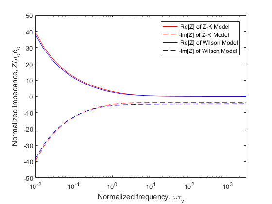
Fig.1. Normalized impedance prediction from the Z-K Model (low frequency) and the Wilson Model. The negative of the imaginary part is plotted. Calculations are shown as a function of the normalized frequency , where is the relaxation time for viscous diffusion in the pores.
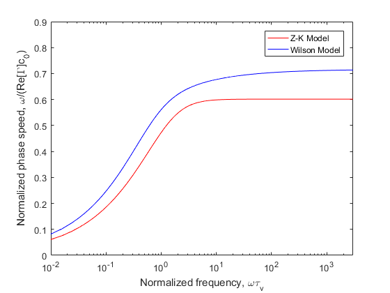
Fig.2. Phase speed predictions from the Z-K Model (low frequency) and the Wilson Model. Plotted is the phase speed divided by the phase speed in air, .
The impedance of two models are nearly identical, but the phase speed of Z-K Model is too low and separate dramatically with the increase of frequency. If we apply high-frequency approximate values of Z-K Model, The continuity equation in will be rewritten as
where is the ratio of specific heats in the air. The impedance and the phase speed of Z-K Model will change a lot as shown in Figs.3-4.
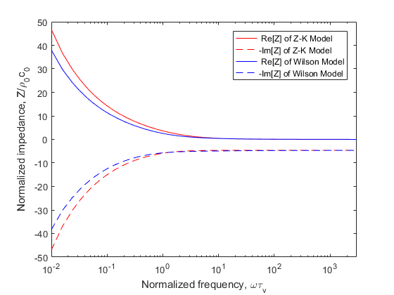
Fig.3. Normalised impedance prediction from the Z-K Model (high frequency) and the Wilson Model. The negative of the imaginary part is plotted. Calculations are shown as a function of the normalised frequency , where is the relaxation time for viscous diffusion in the pores.
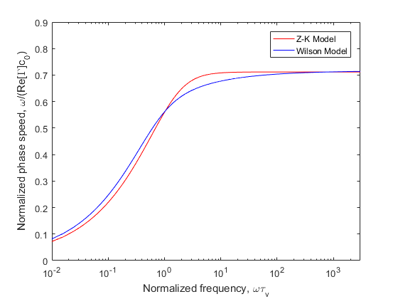
Fig.4. Phase speed predictions from the Z-K Model (high frequency) and the Wilson Model. Plotted is the phase speed divided by the phase speed in air, .
The impedance of the Z-K Model becomes incorrect when , but the phase speed fit better with the Wilson Model. Fig.2 and 4 show that the phase speed becomes independent of frequency for large , whereas it should be actually increase as .
In this section, we consider the time-domain numerical implementation of Z-K equations. For the efficiency of calculation,consider simplify the control equation further:Differentiating the continuity equation in by time, grading the movement equation then one can derive that
That is a single variable control equation which means that one need not consider variable coupling and can improve the efficiency of calculating dramatically. There is a high order spatial term in the control equation. The program uses the idea of shape function to solve it (more detail will be given later). We apply Vertical-Centered Finite Volume Method (VC-FVM) to discrete and define the sound pressure on the mesh node. We assume a linear distribution (or quadratic linear distribution) of the sound pressure within the mesh cell. The control volume of the VC-FVM is showed in Fig.5 (the black lines are the mesh elements and black points are the mesh nodes, the control volume of one example node is surrounded by azure faces) and Fig.6 given the assumption of the sound pressure distribution within the 2-D mesh.
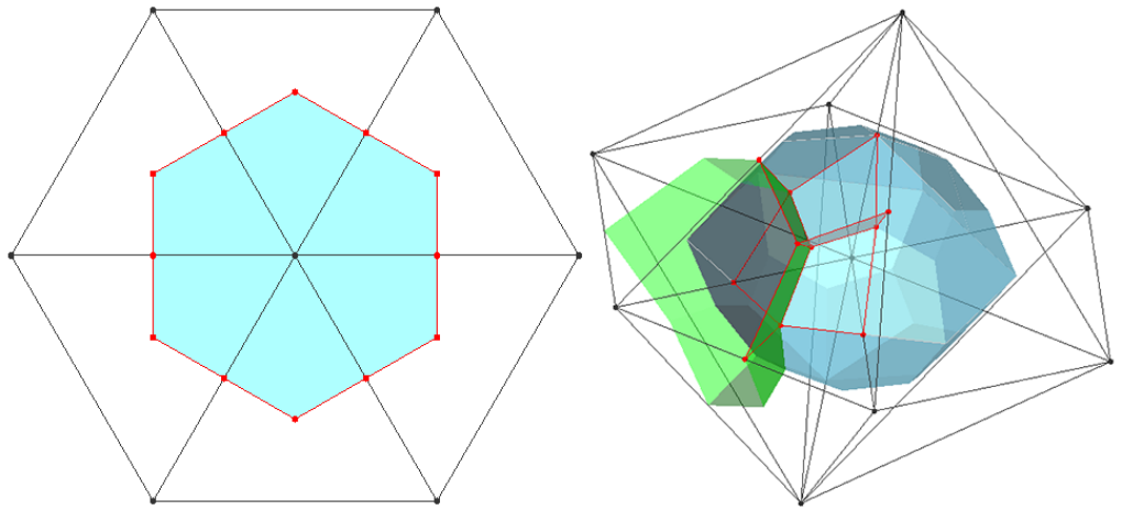
Fig.5. Control volume of the vertex-centred finite volume method (a). 2-D triangle cell (b). 3-D tetrahedron cell.
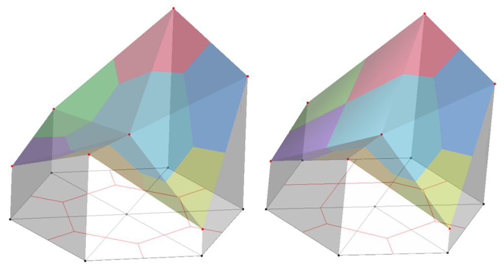
Fig.6. Sound pressure distribution assumed in the 2D mesh, the scale of sound pressure is expressed in height (a). pure triangle cell (b). mixed cell
On any control volume, the integral form of is
Use low order interpolation for the mass term,assume and are uniformly distribution in each control volume as is shown in Fig.7. The discretized equation is
in which , , and refers to the contribution of the area (2-D) or volume (3-D) to that node by the cell.
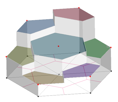
Fig.7. The distribution of sound pressure change rate over time which assumed in the 2-D mesh
We use shape function to calculate the grade of the pressure in the cell,the right side of can be rewritten as
where, and are the shape function of the cell, the value is dependent on the cell shape. In practice, we discrete the time term as
We recalculated a porous triangle barrier given in Ref.13 and the sonic crystals in Ref.9 to test our program. And have made sure that parameter values are the same as each source case, the number of grids in VC-FVM is similar to there source cases.
The Gaussian source was applied as the initial condition, with an expression of
where is the distance from the source position, with in pascals and in meters.
For the air, we have the values of , , the speed of sound of air . When considering the barriers as porous media, we specify the porosity , the static flow resistivity , and the porous medium structure factor , following those specified in Ref.13.
The source is located at (0,1.5)m, and the receiver is located at (9,1)m. Considered the differences between Perfect Matching Layer (PML) and the Clay-Engquist-Majda (C-E-M) boundary, the size of the simulation domain is changed to . We use more dense mesh inside the triangular barrier as is shown in Fig.8. The total cell quantity is 4.5 million, similar to 4.92 million of FDTD. The time step is , and the overall simulation time is . The small grid size warrants a sufficient number of grid nodes within a wavelength, approximately 30 points for the highest frequency of interest at . The small time step not only satisfies the stability condition of the scheme15 and the Nyquist rule for the high-frequency requirement but also gives a low CFL number that is needed to avoid generating spurious waves near the interface between the air and the porous medium.
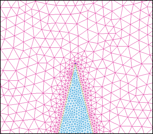
Fig.8. Part of the mesh, the denser mesh was used inside the porous medium.
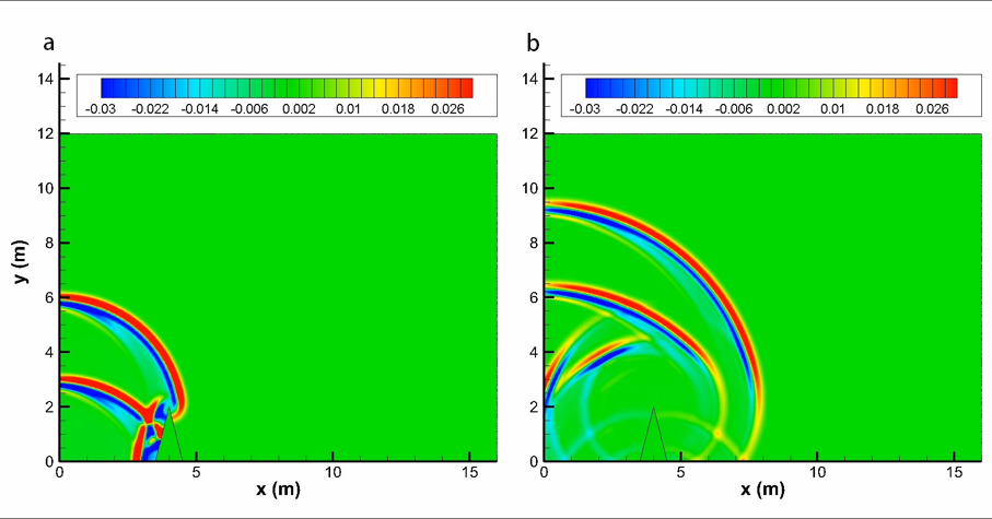
Fig.9. Pressure contours at different times for the single rigid barrier (a). 13 ms (b). 23 ms.
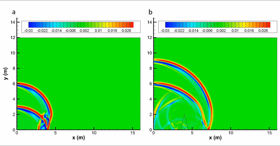
Fig.10. Pressure contours at different times for a triangular porous material barrier with flow resistivity (a). 13 ms (b). 23 ms.
Fig.9 illustrates how sound waves propagate over the single rigid barrier, and Fig.10 shows sound waves penetrate the porous material barrier. To determine the relative sound pressure levels and compare with the FDTD and analytical solutions (only rigid case), we performed a free field computation for sound propagation of the same impulse source to obtain sound pressure and then use the following formula to obtain the relative sound pressure level:
The comparisons with FDTD in time-domain is given in Fig.11, and the corresponding frequency domain contradistinction is given in Fig.12.
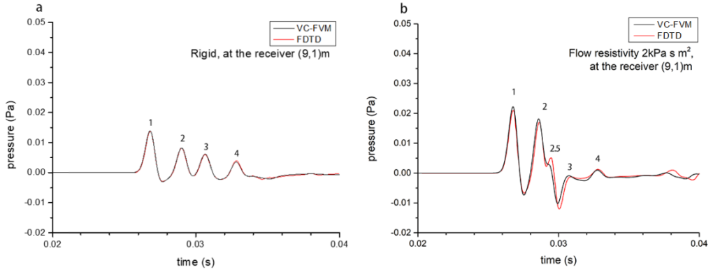
Fig.11. Comparison of time-domain numerical results with FDTD (a). rigid barrier (b). porous material barrier with flow resistivity .
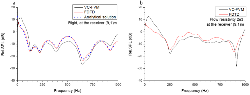
Fig.12. Comparison of frequency domain numerical results with FDTD and analytical solutions (if exist) (a). rigid barrier (b). porous material barrier with flow resistivity .
We numbered some peaks in Fig.11 which you can find corresponding sound pulse propagate route in Fig.13. Most of them fit well with FDTD, but one can find VC-FVM’s “wave 2.5” is propagated faster but weaker than FDTD’s.
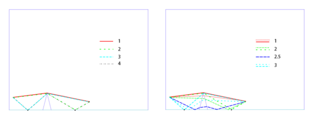
Fig.12. Sound pulse propagate routes (a). rigid barrier (b). porous material barrier with flow resistivity .
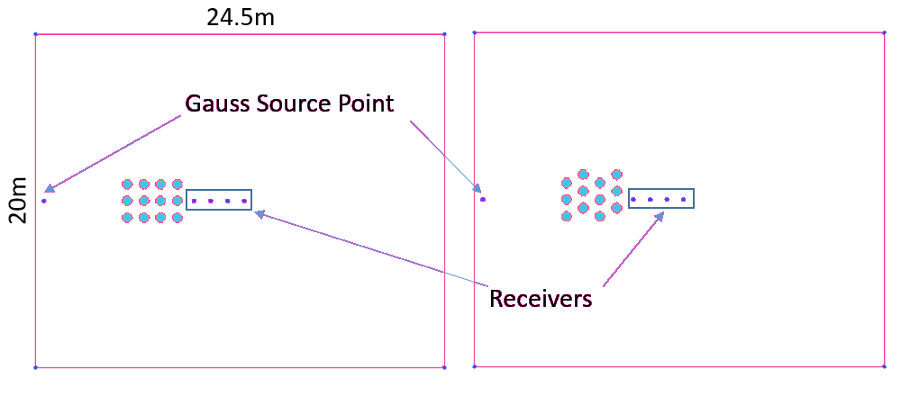
Fig.13. Description of the geometry of the numerical model.
Fig.13 shows the geometry of the numerical model for sound propagation through sonic crystals. The Clay-Engquist-Majda (C-E-M) conditions are specified at all outside boundaries in the cases. The azure zone represents porous medium (parameters are the same with the case triangular barrier). We compared the numerical result of the sound attenuation at the receiver (10,10) as you can see in Fig.14.
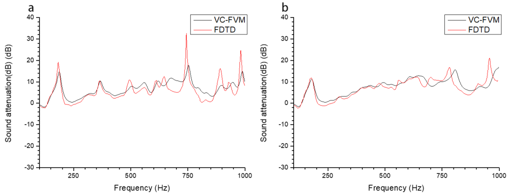
Fig.14. Comparison of the sound attenuation by frequency domain (a). regular square lattice (b). staggered lattice.
[1] Arenas, Jorge P., and Malcolm J. Crocker. “Recent trends in porous sound-absorbing materials.” Sound & vibration 44.7 (2010): 12-18.
[2] Bouakaz, Ayache, Charles T. Lancée, and Nico de Jong. “Harmonic ultrasonic field of medical phased arrays: Simulations and measurements.” IEEE transactions on ultrasonics, ferroelectrics, and frequency control 50.6 (2003): 730-735.
[3] Hallaj, Ibrahim M., and Robin O. Cleveland. “FDTD simulation of finite-amplitude pressure and temperature fields for biomedical ultrasound.” The Journal of the Acoustical Society of America 105.5 (1999): L7-L12.
[4] Jian, X. Q., et al. “FDTD simulation of nonlinear ultrasonic pulse propagation in ESWL.” 2005 IEEE Engineering in Medicine and Biology 27th Annual Conference. IEEE, 2006.
[5] Fukuhara, Keisuke, and Nagayoshi Morita. “FDTD simulation of nonlinear ultrasonic pulse propagation in ESWL using equations including Lagrangian.” Electrical Engineering in Japan 169.4 (2009): 29-36.
[6] Fellah, Z. E. A., and C. Depollier. “Transient acoustic wave propagation in rigid porous media: A time-domain approach.” The Journal of the Acoustical Society of America 107.2 (2000): 683-688.
[7] Miyashita, Toyokatsu, and Chiryu Inoue. “Numerical investigations of transmission and waveguide properties of sonic crystals by finite-difference time-domain method.” Japanese Journal of Applied Physics 40.5S (2001): 3488.
[8] Hu, Xinhua, C. T. Chan, and Jian Zi. “Two-dimensional sonic crystals with Helmholtz resonators.” Physical Review E 71.5 (2005): 055601.
[9] Ke, Guoyi, and Zhongquan Charlie Zheng. “Sound propagation around arrays of rigid and porous cylinders in free space and near a ground boundary.” Journal of Sound and Vibration 370 (2016): 43-53.
[10] Salomons, Erik M., Reinhard Blumrich, and Dietrich Heimann. “Eulerian time-domain model for sound propagation over a finite-impedance ground surface. Comparison with frequency-domain models.” Acta Acustica united with Acustica 88.4 (2002): 483-492.
[11] Wilson, D. Keith, et al. “Time-domain calculations of sound interactions with outdoor ground surfaces.” Applied Acoustics 68.2 (2007): 173-200.
[12] Van Renterghem, Timothy, Dick Botteldooren, and Kris Verheyen. “Road traffic noise shielding by vegetation belts of limited depth.” Journal of Sound and Vibration 331.10 (2012): 2404-2425.
[13] Ke, Guoyi, and Zhongquan Charlie Zheng. “Simulation of sound propagation over porous barriers of arbitrary shapes.” The Journal of the Acoustical Society of America 137.1 (2015): 303-309.
[14] Moukalled, F., L. Mangani, and M. Darwish. “The finite volume method in computational fluid dynamics.” An Advanced Introduction with OpenFOAM and Matlab (2016): 3-8.
[15] Xuan, Ling-kuan, et al. “Time domain finite volume method for three-dimensional structural–acoustic coupling analysis.” Applied Acoustics 76 (2014): 138-149.
]]>With the in-depth study and broad application of acoustic materials, the importance of the characterising acoustic material properties has emerged and risen gradually. The absorption properties and acoustic insulation properties are most used evaluation indexes for acoustic materials. The absorption properties include absorption coefficient and acoustic impedance; the acoustic insulation properties usually evaluated by the transmission losses.
Common acoustic material properties are——Absorption Coefficient, Acoustic Impedance Ratio,Transmission Loss.
There are various methods used to measure and characterise acoustic materials.
To understand and model absorptive materials better, it is necessary to measure materials in a more controlled environment to allow direct comparison between theory and experiment (numerical experiment included).
The steady state pressure in the tube is given by
Where is the a complex constant; is the wave number; R is the the reflection coefficient; is the relative position to the sample. The measurement of the minimum and maximum pressures of the standing wave is needed. The standing wave ratio is defined as the ratio of to and is given by:
The magnitude of the reflection coefficient and the absorption coefficient can be obtained:
One need to measure the distance between where the first minimum pressure appears and the surface of the material to obtain the acoustic impedance ratio :
which is the wave length of the single frequency wave.
Fig.1. Set-ups for impedance tube measurement (Source: Ref. 2)
The standing wave method can only test single frequency waves at a time and need longer tube to test lower frequency wave. By measuring the pressure at two points in the tube the transfer function method can set up and solve simultaneous equations for the reflection coefficient and from there get the impedance and absorption coefficient. This is the principle of the transfer function , often called the two-microphone method.
where,
This method is essentially an adaptation of the transfer function method. It usually use three microphone to cover the frequency range an impedance tube offers.
For most practitioners, the only important measurement is that which gives the random incidence absorption coefficient that is needed for performance specifications in room designing, vegetation belt setting, and so on.
The reverberation chamber test requires large sample sizes and a specialist test room, and so is expensive to undertake. It also only gives absorption coefficients; the impedance cannot be measured. Consequently, developers of absorptive material will often use the impedance tube to build up an understanding of the material properties on small samples, before undertaking reverberation tests.
The reverberation time of a room is dependent on the total absorption in the room. Consequently, by measuring the reverberation time of a room before and after a sample of absorbent is introduced, it is possible to calculate the random incidence absorption coefficient.
The reverberation time before the sample is introduced is given by:
where is the room volume, is the speed of sound, is the average absorption coefficient of the empty room, is the surface area of the room and is the air absorption constant.
The reverberation time after the sample is introduced is given by:
where is the surface area and is the absorption coefficient of the sample. By rearranging Equations and it is possible to obtain the absorption coefficient of the sample.
[1] Chen, ke , xiang . Zeng, and you . Yang. Sheng Xue Ce Liang. Bei jing: Ji xie gong ye chu ban she, 2010. Print.
[2] Cox, Trevor J., and Peter D’Antonio. Acoustic Absorbers and Diffusers: Theory, Design and Application. CRC Press, 2009.
]]>Since the fluid density is always smaller than the frame density in the porous medium, the frame of the porous medium can be seen as motionless (i.e., rigid skeleton porous medium). Special attention has been paid to the propagation of the monochromatic sound wave in the rigid skeleton porous medium. That is because the response of a porous media in the time domain can be described by an instantaneous response and a “susceptibility” kernel responsible for the memory effects. Various empirical and semi-phenomenological models were developed for the describing of the wave propagation in the porous medium. Tab. 1 lists 14 impedance models and the parameters on which they depend.
Tab.1 Impedance models and parameters (adapted from Ref.2).
Model | No. of parameters | Parameters |
---|---|---|
Delany and Bazley (-Miki) | 1 | Effecctive flow resistivity |
Taraldsen | 1 | Effecctive flow resistivity |
Variable porous | 2 | Effecctive flow resistivity, rate of porous variation with depth |
Voronina | 3 | Mean grain dimension, number of grains per unit volume.grain density |
Zwikker and Kosten | 3 | Porosity, flow resistivity, structure factor |
Hamet phenomenological | 3 | Porosity, flow resistivity, structure factor |
Identical tortuous porous | 3 | Porosity, flow resistivity, tortuosity |
Attenborough | 4 | Porosity, flow resistivity, tortuosity, pore shape factor |
Wilson relaxation | 4 | Porosity, tortuosity, Viscous and thermal relaxation times |
Pore size distribution | 4 | Porosity, flow resistivity, tortuosity, distribution parameter |
Johnson/Allard/Umnova | 4 | Porosity, flow resistivity, tortuosity, viscous characteristic lengh |
Johnson/Allard | 5 | Porosity, flow resistivity, tortuosity, viscous, thermal characteristic lengths |
Johnson/Allard/Lafarge | 6 | Porosity, flow resistivity, tortuosity, viscous and thermal characteristic lengths, thermal permeability |
Johnson/Allard/Lafarge/Pride | 8 | Porosity, flow resistivity, tortuosity, viscous and thermal characteristic lengths, thermal permeability, viscous and thermal tortuosity correction factor |
Researchers found that the asymptotic expressions of stiffness and damping in porous medium are proportional to fractional powers of frequency which suggests the fact that time derivatives of fractional order might describe the behavior of the sound waves in this kind of material. Therefore, the time domain expression of sound propagation in porous medium often contains convolution expressions, which makes it difficult for the numerical simulation of the acoustic propagation of porous medium. For example, the Wilson relaxation model can be expressed as:
Here, , , , , is the porosity, is the tortuosity, is the ambient air density. is the ambient air pressure, is the ratio of specific heats, is the Prandtl number and is the pore shape factor. For more details about those parameters one can refer to Ref.3.
The description of sound propagation in the porous medium is often “frequency domain” in commercial software. Though the “frequency domain” argument here is not rigorous. These commercial software solutions are time domain governing equations, but these equations describing monochromatic sounds, and the coefficients in it are frequency dependent. i.e. Zwikker and Kosten model:
Here, is the equivalent density, is the equivalent bulk modulus, they are complex functions of the frequency and of the pore shape.
1 | × Frequency domain: |
As a matter of fact, it is not only the Wilson relaxation model that describes the acoustic propagation of the porous medium in the time-domain. Zwikker & Kosten(1949) has given a time-domain phenomenological model describing the sound propagating in the porous medium:
Here, is the porous structure factor.
Wilson et al.(2007) has pointed out that the ZK phenomenological model captured much of the important physics of sound propagation in porous medium. Theoretically, therefore, ZK phenomenological model is sufficient to meet the kind of simulation like acoustic engineering design calculations.
[1] Fellah, Z. E. A., and C. Depollier. “Transient acoustic wave propagation in rigid porous media: A time-domain approach.” The Journal of the Acoustical Society of America 107.2 (2000): 683-688.
[2] Attenborough, Keith, Imran Bashir, and Shahram Taherzadeh. “Outdoor ground impedance models.” The Journal of the Acoustical Society of America 129.5 (2011): 2806-2819.
[3] Wilson, D. Keith. “Simple, relaxational models for the acoustical properties of porous media.” Applied Acoustics 50.3 (1997): 171-188.
[4] Wilson, D. Keith, et al. “Time-domain calculations of sound interactions with outdoor ground surfaces.” Applied Acoustics 68.2 (2007): 173-200.
[5] Van Renterghem, Timothy, Dick Botteldooren, and Kris Verheyen. “Road traffic noise shielding by vegetation belts of limited depth.” Journal of Sound and Vibration 331.10 (2012): 2404-2425.
]]>Most materials containing pores in them are considered as porous media and porous media widely exist in the world. Basically, a porous medium consists of pore portion and solid matrix or skeletal portion, The porous media in nature are usually filled with liquid or gas. Strictly speaking, most of solid materials in nature are porous media. Fig.1 shows the three main types of porous media, their typical microscopic arrangements and some of the physical models used to describe their mechanisms.
Fig.1. The three main types of porous media (Source: Ref. 2)
With the significant development of the research and applications on porous media in recent years, the concept of porous media can be seen in applying in many areas of applied science and engineering. Wave propagations in porous media have great application significances in the areas of geophysics, earthquake, civil engineering, mechanical engineering, and petroleum engineering.
Due to the fact that the real structure of porous media are very complex, it is impossible to give an exact picture about the phenomenon involving the interaction of fluid and solid surface. To overcome this difficulty, one can treat the porous media as a continuum consisting of series of particles, which is very similar to the definition of fluid density. In other words, people can find a representative volume element of porous media that the size of this volume id required to be much lager than that of a single pore, which indicates that a porous medium contains many pores, which are much less than the characteristic length of the whole flow field. The porous media can then be treated as a continuum consisting of series of such elements.
For certain media, if the porosity is irrelevant to the spatial position, the media are called homogenous media. Otherwise, it is called inhomogeneous media.
The word “fractal” was first introduce by a mathematician, Mandelbrot. The parameter for quantitative description of the property of fractal is called fractal dimension. Contrary to the classical Euclid geometry, whose dimension can only be assigned as an integer because it deals with regular geometrical figures, the dimension of fractal structure is a fraction. The fractal theory is applied to potential regulations from the superficial irregularity and has been widely used among many subjects.
The main characteristics of fractal geometry are self-similar and scale invariant which means part of geometrical shape can be exactly or very close to a reduced size copy of the whole. Actually, it has been reported that the microstructure and the distribution of pore size possess the characteristics of fractal. Sierpinski triangle and Menger sponge, as shown in Fig. 2 and Fig. 3, are typical models usually used in mathematical representing the geometries of porous media.
Fig. 2. Sierpinski triangle (Source: Wikipedia)
Fig. 3. Menger sponge (Source: Wikipedia)
Since the invention of fractal theory, it has been applied to investigate the transportation problem in porous media. The porosity and permeability of porous media may be related to the fractal index.
In investigating wave motions in porous media, the main concern are both the waves regarding the media in which the waves propagate and energy source by which the waves are generated. In fact, the wave motions are affected by a variety of factors such as topologic and material properties of media, characteristics of wave energy sources, medium porosity and permeability, properties of the fluids saturated in the media, as well as combinations of the waves propagation in the domain considered. The behaviors of the wave motions are therefore very complex.
For the media, the wave behavior in a fluid-saturated medium is affected not only by the separate motions of the solid and fluid but also by the relative motion between the solid and fluid. It is generally accepted that the waves attenuate while they propagate in the medium due to the material properties and the presence of the pore fluid in the porous media. In fact, wave velocity and wave attenuation are two key aspects of wave propagation in porous media. These aspects are important in analyzing the dynamic response of the media with respect to the properties of both the media and the wave source, such as viscosity, porosity, and frequency.
For the energy source, the wave propagation described in the governing equations relies on the characteristics of the energy source by which the wave is generated. Therefore, the model describing the wave field with the displacements and relative displacements between the solid and fluid for each point in the porous media domain considered is necessary.
Biot theory describes the elastic waves propagation in a porous saturated medium. Biot ignores the microscopic level and assumes that continuum mechanics can be applied to measurable macroscopic quantities. He postulates the Lagrangian and use Hamilton principle to derive the equations that govern the wave propagation.
The main assumptions of the theory are:
Infinitesimal transformations occur between the reference and current states of deformation. Displacements, strains and particle velocities are small. Consequently, the Eulerian and Lagrangian formulations coincide up to the first-order. The constitutive equations, dissipation forces, and kinetic momenta are linear. (The strain energy, dissipation potential and kinetic energy are quadratic forms in the field variables.)
The principles of continuum mechanics can be applied to measurable macroscopic values. The macroscopic quantities used in Biot’s theory are volume averages of the corresponding microscopic quantities of the constituents.
The wavelength is large compared with the dimensions of a macroscopic elementary volume. This volume has well defined properties, such as porosity, permeability and elastic moduli, which are representative of the medium. Scattering effects are thus neglected.
The conditions are isothermal.
The stress distribution in the fluid is hydrostatic. (It may be not completely hydrostatic, since the fluid is viscous.)
The liquid phase is continuous. The matrix consists of the solid phase and disconnected pores, which do not contribute to the porosity.
In most cases, the material of the frame is isotropic. Anisotropy is due to a preferential alignment of the pores (or cracks).
In engineering applications, the discussion of wave propagations in porous media half-space is often needed. And at a free boundary of half-space, the reflection, refraction and diffraction of the incident wave must be considered. Surely, that would be a difficult subject.
Theoretically, the inhomogeneous wave incident on the boundary of the medium will generate various surface waves.
Rayleigh wave
Fig. 4. The movement of a Rayleigh wave. (Source: quora)
Love wave
Fig. 5. The movement of a Love wave. (Source: quora)
The phenomena describing the reflection, refraction and diffraction of waves are related to the presence of inhomogeneities and interfaces. Knowledge of the corresponding boundary conditions is essential to correctly describe these phenomena. In fluid/fluid contacts in porous materials, we should expect fluid flow across the interface when a wave passes, and as we have mode conversion from P-wave to S-wave energy in single-phase media, we may expect mode conversion between the three waves propagating in a porous medium. In the developments that follow, the following different cases of the appropriate boundary conditions can be derived:
Although numerous investigations have been performed on wave propagations and motions of solid matrix and liquid in the pores, however, there is still a lack of comprehensive understanding on the mechanism of the technique and the mobilization of the fluids in the porous media under the mechanism of the technique and the mobilization of the fluids in the porous media under excitations of the wave motions generated with vibration stimulations.
For further applications, a thorough and systemic study on wave propagations in fluid-saturated porous half-space media in is needed. The progress in such a study will certainly contribute to the comprehensive understanding of the mechanism of the technique and enhance its application.
[1] Hamidzadeh, Hamid R., Liming Dai, and Reza N. Jazar. Wave propagation in solid and porous half-space media. Berlin: Springer, 2014.
[2] Arenas, Jorge P., and Malcolm J. Crocker. “Recent trends in porous sound-absorbing materials.” Sound & vibration 44.7 (2010): 12-18.
[3] Carcione, José M. Wave Fields in Real Media: Wave Propagation in Anisotropic, Anelastic, Porous and Electromagnetic Media. Vol. 38. Elsevier, 2014.
]]>Acoustic waves are small propagating fluctuations in pressure, particle velocity, mass density, entropy and temperature on lager and more uniform background values of these quantities. Let refer to the pressure, partical velocity, mass density, specific entropy density (i.e., entropy per unit mass), and absolute temperature of the background medium, respectively. Then, the total pressure , particle velocity , mass density , specific entropy density , and absolute temperature associated with a propagating acoustic disturbance are assumed to be
Similarly, the total sound speed of the medium is given by
The local form (i.e., the Eulerian specification of the flow field) of the principle of conservation of mass is expressed by the continuity equation (without mass source):
Where the Material Derivative
Movement Equation (or the Equation of momentum) can be derived from the Newton’s Second Law (without body force):
Here denotes the Cauchy stress tensor - a second-order symmetric tensor consisted by 6 independent scalar variables.
The Constitutive Equation explicitly relate the Cauchy stress tensor , the normal stress vector components and the velocity vector component . For isotropic Newtonian fluid, with the Volume viscosity introduced by Stokes in 1949:
Where is the shear viscosity, and is the volume viscosity of the medium. Here we considered the viscous effect of the medium.
Here is the nonlinear coefficient.
Here is the thermal conductivity of the medium.
Here, is the relaxation time, is the sound speed when , is a dimensionless parameter which describing the dispersion and dissipation characteristics of the medium.
It is well know that the Helmholtz Equation is derived from the nonlinear acoustic theories by serial hypothesis. The viscous effect, nonlinear effect, heatconduction effect and relaxation effect can be neglected under these assumptions.
I will discuss when should we apply linear acoustic theory instead of the nonlinear one based on 1-D control equations.
Mach Number is a dimensionless quantity representing the ratio of flow velocity to the local speed of sound.
Where, is the component of total particle velocity
In fluid dynamics, the Reynolds Number is a dimensionless quantity representing the ratio of inertia force to viscous force.
Here, is a characteristic linear dimension. Similarly, we compare the convection term with the dissipative term of the Burgers Equation and got it’s acoustic Reynolds Number. Bugers Equation (no rotation) is derived from the continuity equation, movement equation and the equation of state which considered nonlinear effect and heat conduction effect.
Here, . With the monochromatic traveing wave solution, the acoustic Reynolds Number can be derived
When the backgound medium is stationary, the acoustic Reynolds Number can be write as
If all 3 conditions are met and we can apply linear acoustic theories?
No, the discussion of the relaxiation effect is needed.
[1] Campos, L. M. “On 36 forms of the acoustic wave equation in potential flows and inhomogeneous media.” Applied Mechanics Reviews 60.4 (2007): 149-171.
[2] Qian, zu . Fei Xian Xing Sheng Xue. Bei jing: Ke xue chu ban she, 2009. Print.
[3] Solui︠a︡n, Stepan Ivanovich. Theoretical foundations of nonlinear acoustics. Consultants Bureau, 1977.
]]>I’m the website holder - an undergraduate student who is major in Marine Engineering at Harbin Engineering University. I’ll post some excerpts or reviews of the fields what am I interested in. The site is serving as an academic information memo of mine.
Thanks for visiting 😉
]]>